The MiraiShield Project
Inspiration
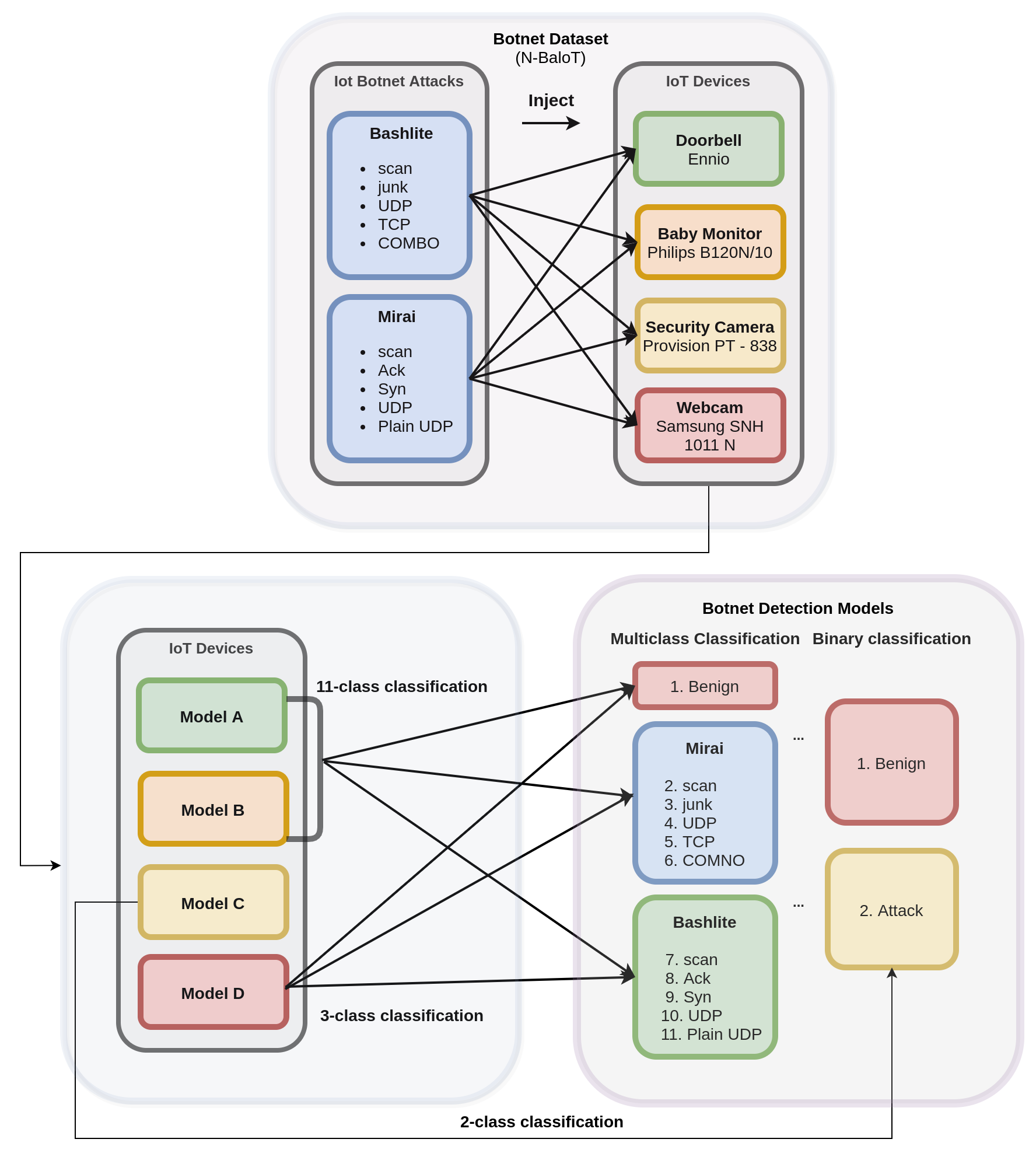
Billions of devices are connected to the internet, and the applications of these devices are booming exponentially. This number is estimated to grow five-fold in the next couple of years. If anything can stop IoT from taking over humanity, it is the security issues that arise with its public usage. Various malwares like the Mirai malware can take down a network and the current methods are not very effective against it. We have shown how a Deep learning model can tackle these threats.
What is Mirai?
Mirai is a vicious malware that turns any IoT network into a network controlled by bots. This network of bots is called Botnet and this Botnet is used to disrupt the traffic of the network by overwhelming the network with a flood of requests. This is called distributed denial-of-service (DDoS) attack. If the default username and password is not changed, Mirai can log into the network and attack it.
What is Bashlite?
Bashlite was used in large-scale DDoS attacks in 2014, but it has since crossed over to infecting IoT devices. In its previous iterations, Bashlite exploited Shellshock to gain a foothold into the vulnerable devices. An attacker can then remotely issue commands particularly, to launch DDoS attacks, and download other files to the compromised devices.
Deep Learning
Deep learning is a subdomain of Machine Learning (ML) that uses Neural networks. If we analyse the network traffic, we’ll be able to find which is Mirai attack and which is not. Lets say a network receives x requests per second normally. If it suddenly receives 2000x requests per second continuously, we can conclude its due to Mirai. So, if we’re given the data about the network traffic, we can use that data to train a deep learning model to tell if it’s infected by Mirai or not.
In order to pre-train our model, we used an open-sourced dataset. The Keras-like code has been demonstrated in this documentation, which can further be utilised.
Training the Model
A Visual representation of the models
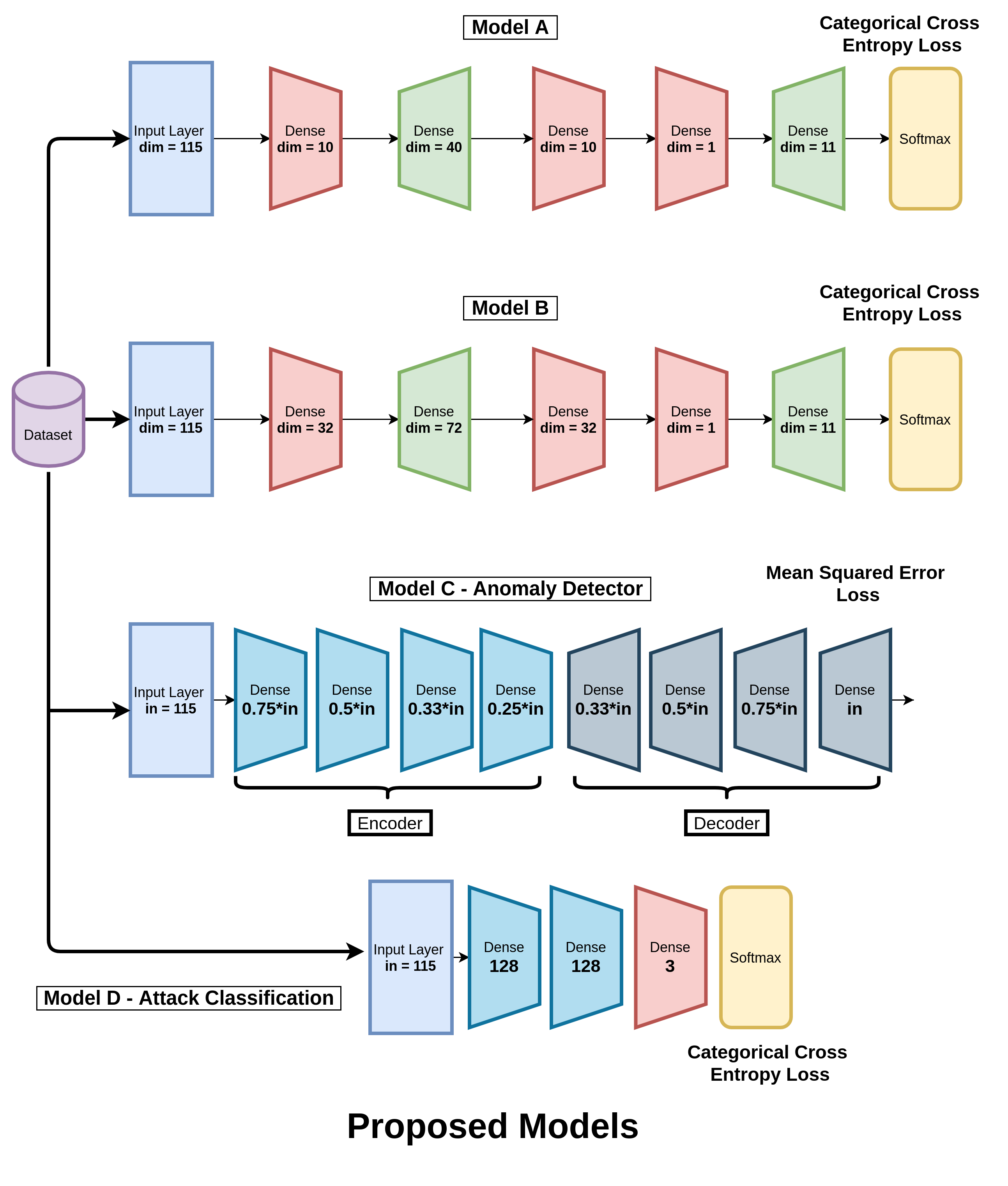
Model A
We created a neural network with input layer of dimension 115 and then subsequent dense layers of dimensions 10, 40, 10, 1, 11 followed by a Softmax activation function.
Model B
This time we created a neural network with input layer of dimension 115 and then subsequent dense layers of dimensions 32, 72, 32, 1, 11 followed by a Softmax activation function.
Models A and B are just an intelligent combination of multiple stages composed of upsampling and downsampling the feature space in order to simulate an expand-reduce transformation. This heuristic of designing our model does not perform as well as we require it to, as some information involving correlation between different features in the hidden dimensions is lost. Additionally, in the end, we apply a Softmax layer to obtain the probability distribution amongst all the 11 classes for easy classification into benign and the multiple sub-classes of malicious.
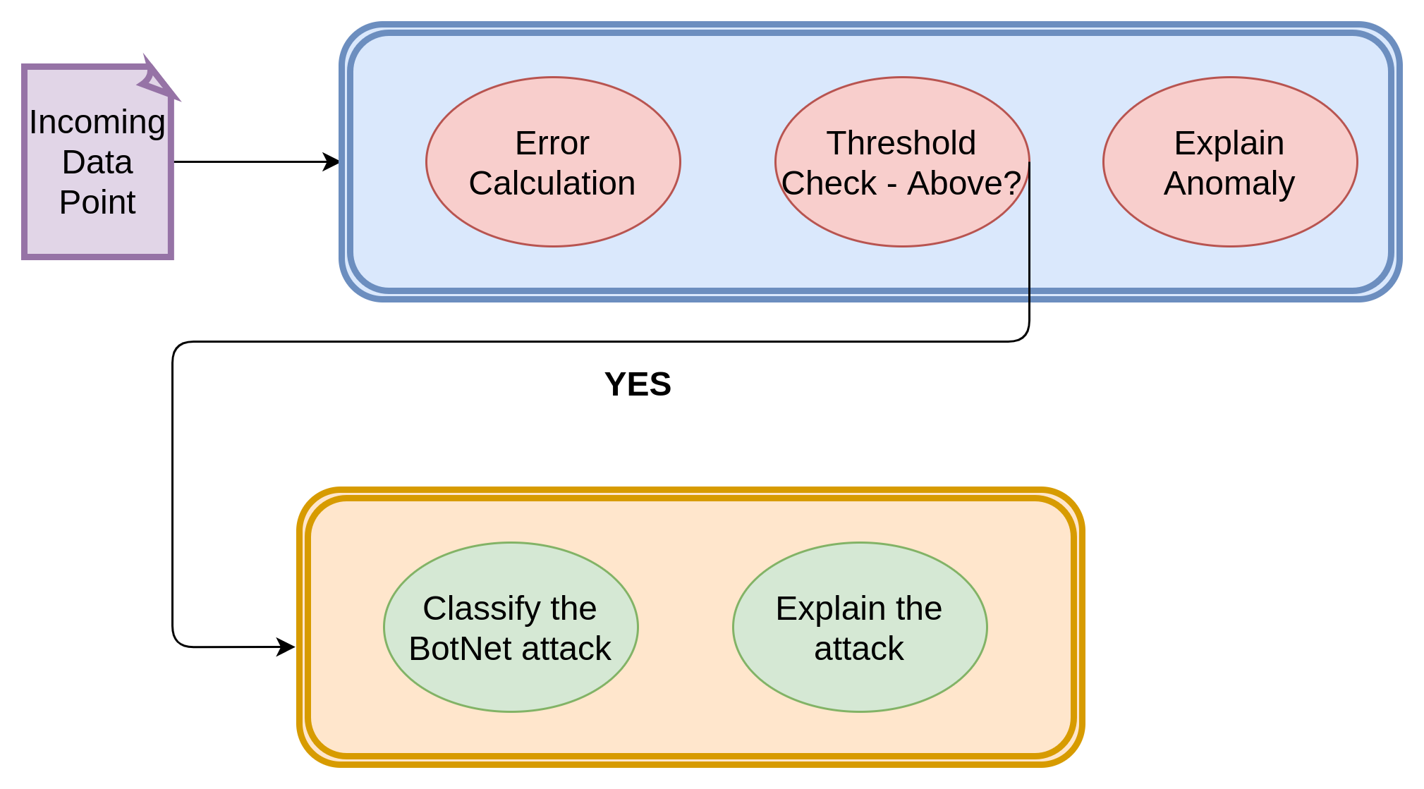
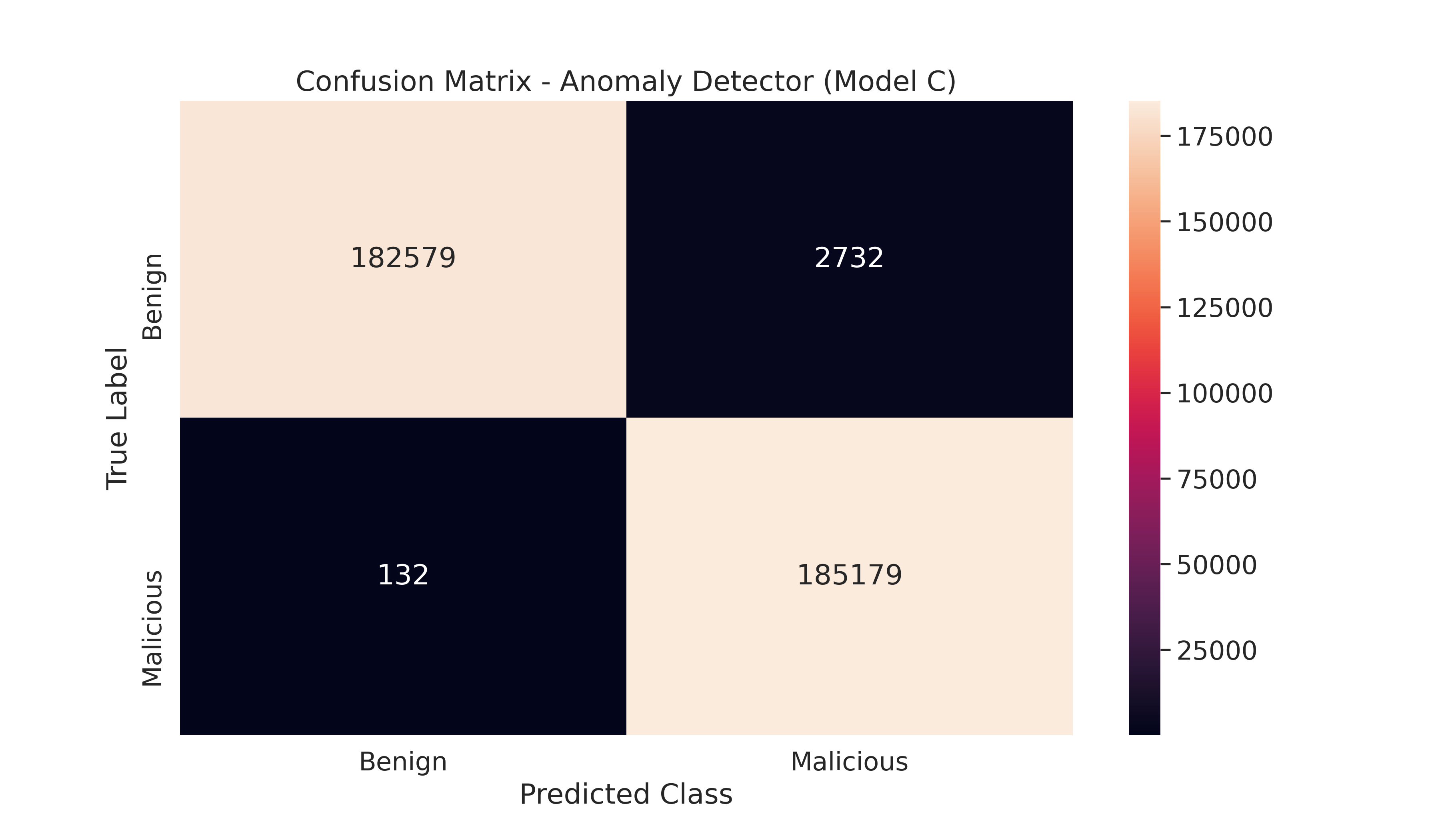
Model C - Benign vs Malicious - Anomaly Detector
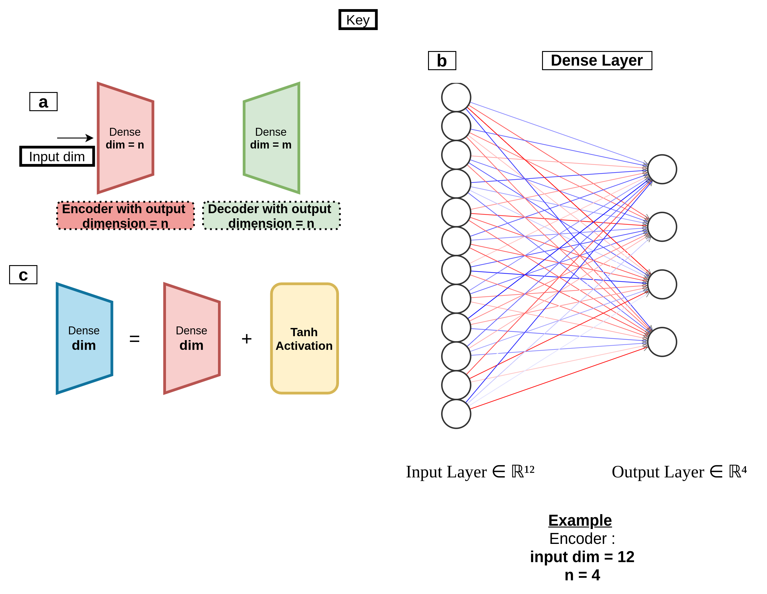
An autoencoder is a neural network trained to reconstruct its inputs after they have been compressed. It consists of an encoder and a decoder part, which each consists of Linear layers in our case. The compression ensures that the network learns meaningful concepts, mainly the relationships between its input features. If we train the autoencoder solely on benign instances, it will successfully reconstruct normal observations but fail to reconstruct abnormal observations.
When a significant reconstruction error has been calculated, the given observations are classified as an anomaly. We optimize the parameters and hyperparameters of each trained model so that when applied to unseen traffic, the model maximizes the true positive rate (correctly marking benign data) and minimizes the false positive rate (wrongly marking benign data as malicious).
The Keras Deep Learning framework was used for modeling and evaluation in Python. This model is used to classify the collected data points into Benign or a Malicious Attack.
The code:
# Initial Python package imports
import sys
import os
import pandas as pd
from glob import iglob
import numpy as np
from keras.models import load_model
import tensorflow as tf
from sklearn.preprocessing import StandardScaler

# Keras imports
from keras.models import Model, Sequential
from keras.layers import Input, Dense
from keras.callbacks import ModelCheckpoint, TensorBoard
from keras.optimizers import SGD

def train(top_n_features=10):

    scaler = StandardScaler()
    scaler.fit(x_train.append(x_opt))
    x_train = scaler.transform(x_train)
    x_opt = scaler.transform(x_opt)
    x_test = scaler.transform(x_test)

    model = autoenc_model(top_n_features)
    model.compile(loss="mean_squared_error",
                    optimizer="sgd")
    cp = ModelCheckpoint(filepath=f"models/model_{top_n_features}.h5",
                               save_best_only=True,
                               verbose=0)
    tb = TensorBoard(log_dir=f"./logs",
                histogram_freq=0,
                write_graph=True,
                write_images=True)

    # Train the model
    model.fit(x_train, x_train,
                    epochs=500,
                    batch_size=64,
                    validation_data=(x_opt, x_opt),
                    verbose=1,
                    callbacks=[cp, tb])

    x_opt_predictions = model.predict(x_opt)
    mse = np.mean(np.power(x_opt - x_opt_predictions, 2), axis=1)
    print("Mean is %.5f" % mse.mean())
    print("Min is %.5f" % mse.min())
    print("Max is %.5f" % mse.max())
    print("Std is %.5f" % mse.std())


    error_dev = mse.mean() + mse.std()

    with open(f'threshold_{top_n_features}', 'w') as t:
        t.write(str(error_dev))
    print(f"Threshold is {error_dev}")

    x_test_predictions = model.predict(x_test)
    print("MSE on the test set")
    mse_test = np.mean(np.power(x_test - x_test_predictions, 2), axis=1)
    over_ed = mse_test > error_dev
    false_positives = sum(over_ed)
    test_size = mse_test.shape[0]
    print(f"{false_positives} FP on the dataset without attacks - size {test_size}")


def autoenc_model(input_dim):
    autoencoder = Sequential()
    autoencoder.add(Dense(int(0.75 * input_dim), activation="tanh", input_shape=(input_dim,)))
    autoencoder.add(Dense(int(0.5 * input_dim), activation="tanh"))
    autoencoder.add(Dense(int(0.33 * input_dim), activation="tanh"))
    autoencoder.add(Dense(int(0.25 * input_dim), activation="tanh"))
    autoencoder.add(Dense(int(0.33 * input_dim), activation="tanh"))
    autoencoder.add(Dense(int(0.5 * input_dim), activation="tanh"))
    autoencoder.add(Dense(int(0.75 * input_dim), activation="tanh"))
    autoencoder.add(Dense(input_dim))
    return autoencoder

if __name__ == "__main__":
    train()
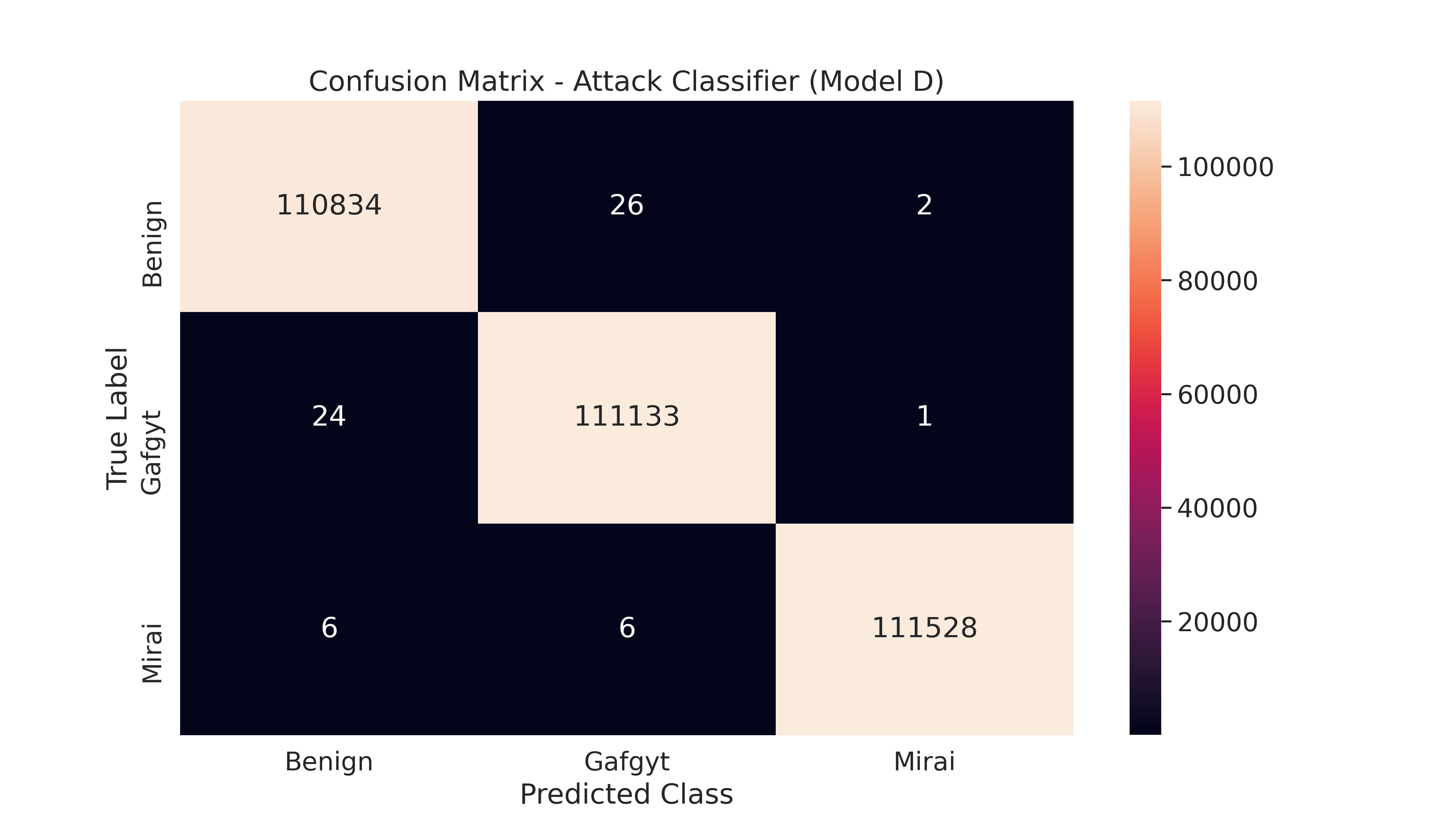
Model D - Benign vs Mirai vs Bashlite - Attack Classifier
This model is used to classify the given attack into Benign, Mirai or Gafgyt (Bashlite).
The code:
# Python Imports

import sys
import os
from glob import iglob
import pandas as pd
import numpy as np
import tensorflow as tf
import pickle

# Scikit-learn imports
from sklearn.preprocessing import StandardScaler
from sklearn.metrics import confusion_matrix
from sklearn.model_selection import train_test_split

# Keras imports
from keras.models import model_from_yaml
from keras.models import Model, Sequential
from keras.layers import Input, Dense, Activation
from keras.callbacks import ModelCheckpoint, TensorBoard
from keras.optimizers import Adam


def create_model(input_dim, add_hidden_layers, hidden_layer_size):
    model = Sequential()
    model.add(Dense(hidden_layer_size, activation="tanh", input_shape=(input_dim,)))
    for i in range(add_hidden_layers):
        model.add(Dense(hidden_layer_size, activation="tanh"))
    model.add(Dense(3))
    model.add(Activation('softmax'))
    return model

def train(top_n_features = None):
    df = load_data()
    train_with_data(top_n_features, df)

def train_with_data(top_n_features = None, df = None):
    X = df.drop(columns=['class'])
    if top_n_features is not None:
        fisher = pd.read_csv('/content/botnet-traffic-analysis/data/top_features_fisherscore.csv')
        features = fisher.iloc[0:int(top_n_features)]['Feature'].values
        X = X[list(features)]
    Y = pd.get_dummies(df['class'])
    print('Splitting data')
    x_train, x_test, y_train, y_test = train_test_split(X, Y, test_size=0.2, random_state=42)
    scaler = StandardScaler()
    print('Transforming data')
    scaler.fit(x_train)
    input_dim = X.shape[1]
    scalerfile = f'./models/scaler_{input_dim}.sav'
    pickle.dump(scaler, open(scalerfile, 'wb'))
    x_train = scaler.transform(x_train)
    x_test = scaler.transform(x_test)
    print('Creating a model')

    model = create_model(input_dim, 1, 128)
    model.compile(loss='categorical_crossentropy', optimizer='adam', metrics=['accuracy'])
    cp = ModelCheckpoint(filepath=f'./models/model_{input_dim}.h5',
                               save_best_only=True,
                               verbose=0)
    tb = TensorBoard(log_dir=f'./logs',
                histogram_freq=0,
                write_graph=True,
                write_images=True)
    epochs = 25
    model.fit(x_train, y_train,
                    epochs=epochs,
                    batch_size=256,
                    validation_data=(x_test, y_test),
                    verbose=1,
                    callbacks=[tb, cp])

if __name__ == "__main__":
    train()
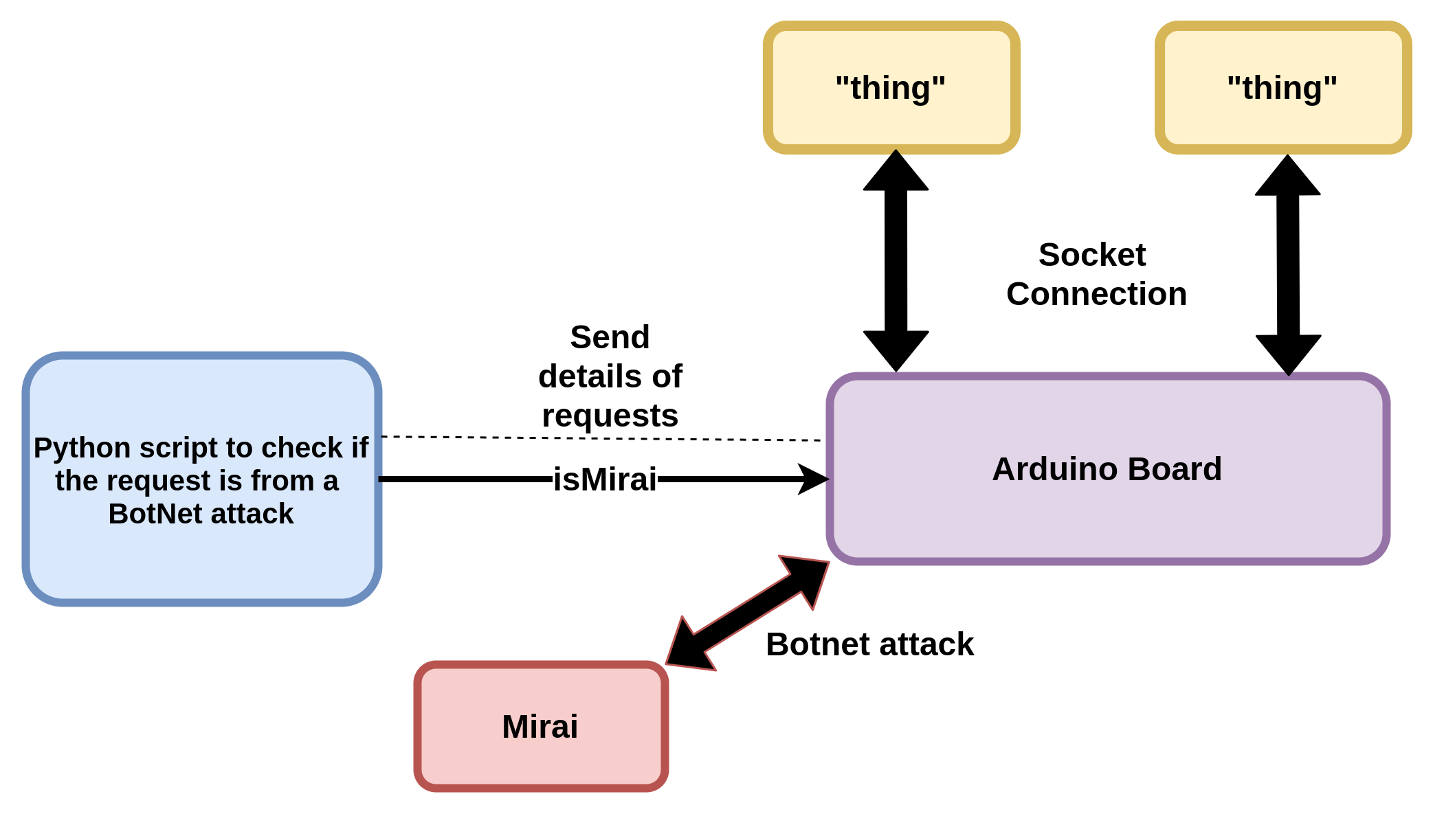
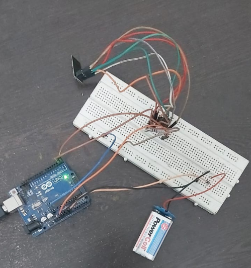
The below diagrams represent the Hardware Flow and our Setup. We will be uploading the final video shortly. In the video below, you can observe the functioning of all 4 models. We have implemented Model A and B for exhaustive purposes of finding the subclass of BotNet attack, Model C for the detection of an anomaly, and Model D for the classification of an attack into its major classes of Benign, Mirai and Bashlite.
You can watch our Video Demonstration of the models we designed here! Just click on the video.
The Hardware Code:
#include <ESP8266WiFi.h>
#include <ESPAsyncTCP.h>
#include <ESPAsyncWebServer.h>


const char* ssid = "REPLACE_WITH_YOUR_SSID";
const char* password = "REPLACE_WITH_YOUR_PASSWORD";

bool ledState = 0;
const int ledPin = 2;

AsyncWebServer server(80);
AsyncWebSocket ws("/ws");


time_t current_time;

const char* key = "vskvskbvskbvjskdbvk";
const AsyncWebSocketClient *script;

void notifyClients() {
  ws.textAll(String(ledState));
}

void handleWebSocketMessage(void *arg, uint8_t *data, size_t len,AsyncWebSocketClient *client) {
  AwsFrameInfo *info = (AwsFrameInfo*)arg;
  if (info->final && info->index == 0 && info->len == len && info->opcode == WS_TEXT) {
    data[len] = 0;
    if(strcmp(data,key)==0){
      script = client;
    }

    Serial.printf(data);


  }
}

void onEvent(AsyncWebSocket *server, AsyncWebSocketClient *client, AwsEventType type,
             void *arg, uint8_t *data, size_t len) {
    ws.text(script)(String(current_time,client));
    if(client == script){
      if(data){
        Serial.printf("Mirai Detected!");
        digitalWrite(ledPin, HIGH);
      }
    }
    switch (type) {
      case WS_EVT_CONNECT:
        Serial.printf("WebSocket client #%u connected from %s\n", client->id(), client->remoteIP().toString().c_str());
        break;
      case WS_EVT_DISCONNECT:
        Serial.printf("WebSocket client #%u disconnected\n", client->id());
        break;
      case WS_EVT_DATA:
        handleWebSocketMessage(arg, data, len,client);
        break;
      case WS_EVT_PONG:
      case WS_EVT_ERROR:
        break;
  }
}

void initWebSocket() {
  ws.onEvent(onEvent);
  server.addHandler(&ws);
}


void setup(){
  Serial.begin(115200);
  current_time = time(NULL);

  pinMode(ledPin, OUTPUT);
  digitalWrite(ledPin, LOW);

  WiFi.begin(ssid, password);
  while (WiFi.status() != WL_CONNECTED) {
    delay(1000);
    Serial.println("Connecting to WiFi..");
  }


  Serial.println(WiFi.localIP());

  initWebSocket();

  server.on("/", HTTP_GET, [](AsyncWebServerRequest *request){
    request->send_P(200);
  });

  server.begin();
}

void loop() {
  ws.cleanupClients();
  digitalWrite(ledPin, ledState);
}
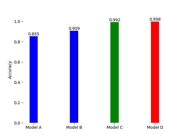
Result
The accuracies of our models are shown below:
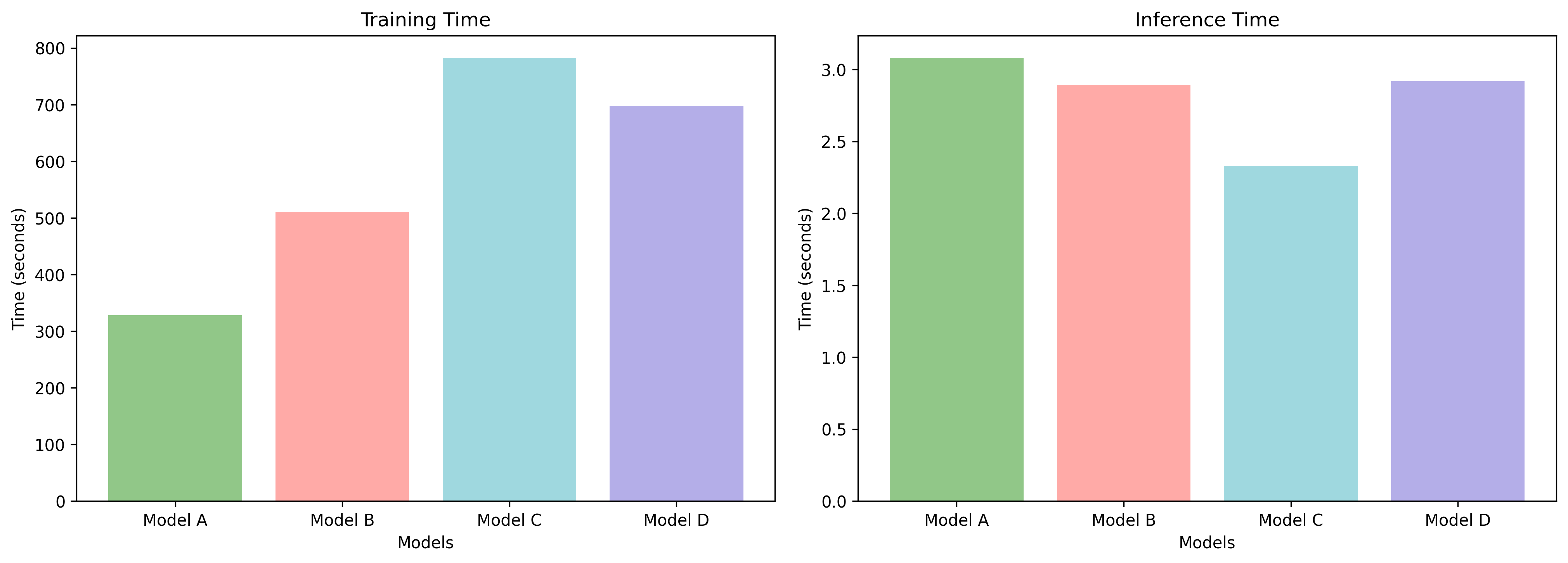
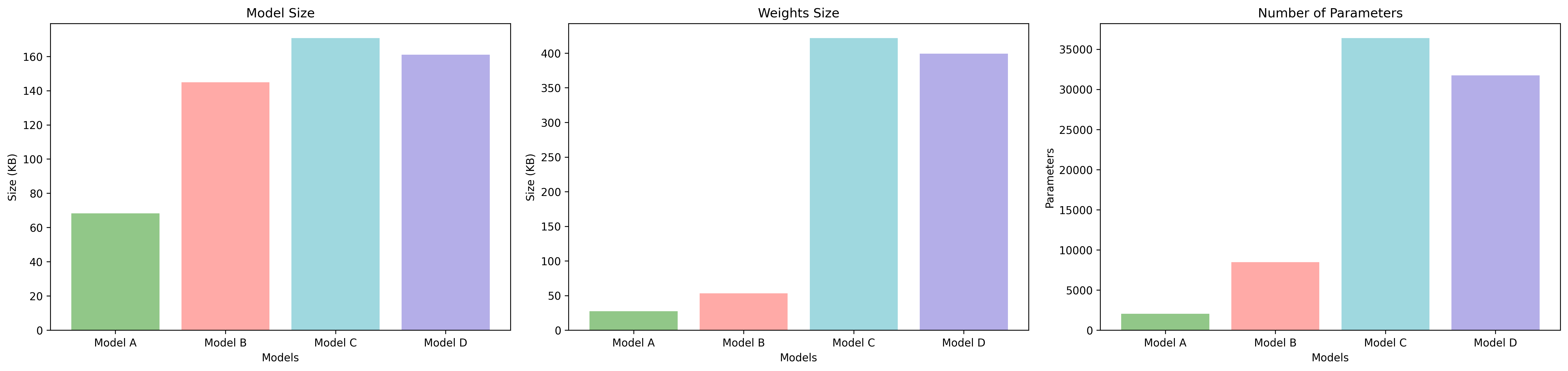
We plot the Training time, Inference time and Model Sizes as shown below. We can observe that all 4 models we have designed can be implemented in real-time, since they have a low inference time and small size in the order of KiloBytes. Hence, the model can be deployed on the cloud, and even on edge devices using Tensorflow Lite.
References
@misc{Dua:2019 ,
author = "Dua, Dheeru and Graff, Casey",
year = "2017",
title = "{UCI} Machine Learning Repository",
url = "http://archive.ics.uci.edu/ml",
institution = "University of California, Irvine, School of Information and Computer Sciences" }
@ARTICLE{8490192,
author={Meidan, Yair and Bohadana, Michael and Mathov, Yael and Mirsky, Yisroel and Shabtai, Asaf and Breitenbacher, Dominik and Elovici, Yuval},
journal={IEEE Pervasive Computing},
title={N-BaIoT—Network-Based Detection of IoT Botnet Attacks Using Deep Autoencoders},
year={2018},
volume={17},
number={3},
pages={12-22},
doi={10.1109/MPRV.2018.03367731}}